Heron Formula
by R. Grothmann
We compute the area of a triangle with sides a, b and c. First set points into (0,0), (a,0) and (x,y), which form such a triangle. I.e., we solve
![]()
for x and y.
>sol &= solve([x^2+y^2=b^2,(x-a)^2+y^2=c^2],[x,y])
                2    2    2
             - c  + b  + a
       [[x = --------------, y =
                  2 a
          4      2  2      2  2    4      2  2    4
  sqrt(- c  + 2 b  c  + 2 a  c  - b  + 2 a  b  - a )
- --------------------------------------------------],
                         2 a
        2    2    2
     - c  + b  + a
[x = --------------, y =
          2 a
        4      2  2      2  2    4      2  2    4
sqrt(- c  + 2 b  c  + 2 a  c  - b  + 2 a  b  - a )
--------------------------------------------------]]
                       2 a
Extract the solution y.
>ysol &= y with sol[2][2]
                  4      2  2      2  2    4      2  2    4
          sqrt(- c  + 2 b  c  + 2 a  c  - b  + 2 a  b  - a )
          --------------------------------------------------
                                 2 a
We get the Heron formula.
>function F(a,b,c) &= sqrt(factor((ysol*a/2)^2))
       sqrt((- c + b + a) (c - b + a) (c + b - a) (c + b + a))
       -------------------------------------------------------
                                  4
Of course, each rectangular triangle is a well known case.
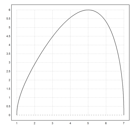
>F(3,4,5)
6
And it is also obvious, that this is the triangle with maximal area and the two sides 3 and 4.
>plot2d(&F(3,4,x),1,7):
The general case works too.
>&solve(diff(F(a,b,c)^2,c)=0,c)
                        2    2             2    2
           [c = - sqrt(b  + a ), c = sqrt(b  + a ), c = 0]
Now let us find the set of all points where b+c=d for some constant d. It is well known that this is an ellipse.
>s1 &= subst(d-c,b,sol[2])
                   2    2    2
            (d - c)  - c  + a
       [x = ------------------, y =
                   2 a
               4      2        2      2        2    4      2  2    4
 sqrt(- (d - c)  + 2 c  (d - c)  + 2 a  (d - c)  - c  + 2 a  c  - a )
 --------------------------------------------------------------------]
                                 2 a
And make functions of this.
>function fx(a,c,d) &= rhs(s1[1]), function fy(a,c,d) &= rhs(s1[2])
                                 2    2    2
                          (d - c)  - c  + a
                          ------------------
                                 2 a


                4      2        2      2        2    4      2  2    4
  sqrt(- (d - c)  + 2 c  (d - c)  + 2 a  (d - c)  - c  + 2 a  c  - a )
  --------------------------------------------------------------------
                                  2 a
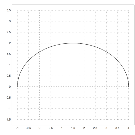
Now we can draw the set. The side b varies from 1 to 4. It is well known that we get an ellipse.
>plot2d(&fx(3,x,5),&fy(3,x,5),xmin=1,xmax=4,square=1):
We can check the general equation for this ellipse, i.e.
![]()
where (xm,ym) is the center, and u and v are the half axes.
>&ratsimp((fx(a,c,d)-a/2)^2/u^2+fy(a,c,d)^2/v^2 with [u=d/2,v=sqrt(d^2-a^2)/2])
1
We see that the height and thus the area of the triangle is maximal for x=0. Thus the area of a triangle with a+b+c=d is maximal, if it is equilateral. We wish to derive this analytically.
>eqns &= [diff(F(a,b,d-(a+b))^2,a)=0,diff(F(a,b,d-(a+b))^2,b)=0]
        d (d - 2 a) (d - 2 b)   (- d + 2 b + 2 a) d (d - 2 b)
       [--------------------- - ----------------------------- = 0,
                  8                           8
            d (d - 2 a) (d - 2 b)   (- d + 2 b + 2 a) d (d - 2 a)
            --------------------- - ----------------------------- = 0]
                      8                           8
We get some minima, which belong to triangles with one side 0, and the solution a=b=c=d/3.
>&solve(eqns,[a,b])
             d      d               d        d
       [[a = -, b = -], [a = 0, b = -], [a = -, b = 0],
             3      3               2        2
                                                            d      d
                                                       [a = -, b = -]]
                                                            2      2
There is also the Lagrange method, maximizing F(a,b,c)^2 with respect to a+b+d=d.
>&solve([diff(F(a,b,c)^2,a)=la,diff(F(a,b,c)^2,b)=la, ...
    diff(F(a,b,c)^2,c)=la,a+b+c=d],[a,b,c,la])
                    d      d                d             d
       [[a = 0, b = -, c = -, la = 0], [a = -, b = 0, c = -, la = 0],
                    2      2                2             2
                                                                  3
            d      d                       d      d      d       d
       [a = -, b = -, c = 0, la = 0], [a = -, b = -, c = -, la = ---]]
            2      2                       3      3      3       108
We can make a plot of the situation with the utility functions in geometry.e.
>load geometry;
First set the points in Maxima.
>A &= at([x,y],sol[2])
            2    2    2
         - c  + b  + a
        [--------------,
              2 a
                           4      2  2      2  2    4      2  2    4
                   sqrt(- c  + 2 b  c  + 2 a  c  - b  + 2 a  b  - a )
                   --------------------------------------------------]
                                          2 a
>B &= [0,0], C &= [a,0]
                                [0, 0]


                                [a, 0]
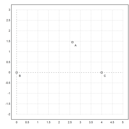
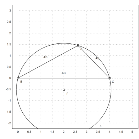
Then set the plot range, and plot the points.
>setPlotRange(0,5,-2,3); ...
 a=4; b=3; c=2; ...
 plotPoint(mxmeval("B"),"B"); plotPoint(mxmeval("C"),"C"); ...
 plotPoint(mxmeval("A"),"A"):
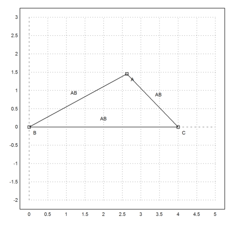
Plot the segments.
>plotSegment(mxmeval("A"),mxmeval("C")); ...
 plotSegment(mxmeval("B"),mxmeval("C")); ...
 plotSegment(mxmeval("B"),mxmeval("A")):
Compute the middle perpendicular in Maxima.
>h &= middlePerpendicular(A,B); g &= middlePerpendicular(B,C);
And the center of the circumference.
>U &= lineIntersection(h,g);
We get the formula for the radius of the circumcircle.
>&assume(a>0,b>0,c>0); & distance(U,B) | radcan
                                   I a b c
       ---------------------------------------------------------------
       sqrt(c - b - a) sqrt(c - b + a) sqrt(c + b - a) sqrt(c + b + a)
Let us add this to the plot.
>plotPoint(U()); ...
 plotCircle(circleWithCenter(mxmeval("U"),mxmeval("distance(U,C)"))):
Using geometry, we derive the simple formula
![]()
for the radius. We can check, if this is really true with Maxima. Maxima will factor this only if we square it.
>& c^2/sin(computeAngle(A,B,C))^2 | factor
                                 2  2  2
                              4 a  b  c
          - -----------------------------------------------
            (c - b - a) (c - b + a) (c + b - a) (c + b + a)